

When the Fed raises rates of interest, how does inflation reply? Are there “lengthy and variable lags” to inflation and output?
There’s a customary story: The Fed raises rates of interest; inflation is sticky so actual rates of interest (rate of interest – inflation) rise; larger actual rates of interest decrease output and employment; the softer economic system pushes inflation down. Every of those is a lagged impact. However regardless of 40 years of effort, principle struggles to substantiate that story (subsequent submit), it is needed to see within the knowledge (final submit), and the empirical work is ephemeral — this submit.
The vector autoregression and associated native projection are immediately the usual empirical instruments to handle how financial coverage impacts the economic system, and have been since Chris Sims’ nice work within the Seventies. (See Larry Christiano’s evaluate.)
I’m dropping religion within the technique and outcomes. We have to discover new methods to study concerning the results of financial coverage. This submit expands on some ideas on this matter in “Expectations and the Neutrality of Curiosity Charges,” a number of of my papers from the Nineties* and wonderful current opinions from Valerie Ramey and Emi Nakamura and Jón Steinsson, who eloquently summarize the laborious identification and computation troubles of up to date empirical work.
Perhaps fashionable knowledge is correct, and economics simply has to catch up. Maybe we’ll. However a preferred perception that doesn’t have strong scientific principle and empirical backing, regardless of a 40 yr effort for fashions and knowledge that may present the specified reply, should be a bit much less reliable than one which does have such foundations. Sensible individuals ought to take into account that the Fed could also be much less highly effective than historically thought, and that its rate of interest coverage has completely different results than generally thought. Whether or not and underneath what circumstances excessive rates of interest decrease inflation, whether or not they achieve this with lengthy and variable however nonetheless predictable and exploitable lags, is way much less sure than you assume.
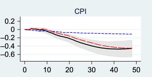
The black strains plot the unique specification. The highest left panel plots the trail of the Federal Funds price after the Fed unexpectedly raises the rate of interest. The funds price goes up, however just for 6 months or so. Industrial manufacturing goes down and unemployment goes up, peaking at month 20. The determine plots the stage of the CPI, so inflation is the slope of the decrease proper hand panel. You see inflation goes the “improper” manner, up, for about 6 months, after which gently declines. Rates of interest certainly appear to have an effect on the economic system with lengthy lags.
This was the broad define of consensus empirical estimates for a few years. It is not uncommon to many different research, and it’s in step with the beliefs of coverage makers and analysts. It is just about what Friedman (1968) advised us to count on. Getting modern fashions to provide one thing like that is a lot more durable, however that is the following weblog submit.
I attempt to hold this weblog accessible to nonspecialists, so I will step again momentarily to elucidate how we produce graphs like these. Economists who know what a VAR is ought to skip to the following part heading.
How can we measure the impact of financial coverage on different variables? Milton Friedman and Anna Schwartz kicked it off within the Financial Historical past by pointing to the historic correlation of cash progress with inflation and output. They knew as we do this correlation is just not causation, in order that they pointed to the truth that cash progress preceeded inflation and output progress. However as James Tobin identified, the cock’s crow comes earlier than, however doesn’t trigger, the solar to rise. So too individuals might go get out some cash forward of time after they see extra future enterprise exercise on the horizon. Even correlation with a lead is just not causation. What to do? Clive Granger’s causality and Chris Sims’ VAR, particularly “Macroeconomics and Actuality” gave immediately’s reply. (And there’s a purpose that everyone talked about up to now has a Nobel prize.)
First, we discover a financial coverage “shock,” a motion within the rate of interest (lately; cash, then) that’s plausibly not a response to financial occasions and particularly to anticipated future financial occasions. We consider the Fed setting rates of interest by a response to financial knowledge plus deviations from that response, equivalent to
rate of interest = (#) output + (#) inflation + (#) different variables + disturbance.
We wish to isolate the “disturbance,” actions within the rate of interest not taken in response to financial occasions. (I exploit “shock” to imply an unpredictable variable, and “disturbance” to imply deviation from an equation just like the above, however one that may persist for some time. A financial coverage “shock” is an surprising motion within the disturbance.) The “rule” half right here will be however needn’t be the Taylor rule, and might embody different variables than output and inflation. It’s what the Fed often does given different variables, and due to this fact (hopefully) controls for reverse causality from anticipated future financial occasions to rates of interest.
Now, in any particular person episode, output and inflation and inflation following a shock will probably be influenced by subsequent shocks to the economic system, financial and different. However these common out. So, the common worth of inflation, output, employment, and so on. following a financial coverage shock is a measure of how the shock impacts the economic system all by itself. That’s what has been plotted above.
VARs had been one of many first large advances within the trendy empirical quest to search out “exogenous” variation and (considerably) credibly discover causal relationships.
Largely the massive literature varies on how one finds the “shocks.” Conventional VARs use regressions of the above equations and the residual is the shock, with a giant query simply what number of and which contemporaneous variables one provides within the regression. Romer and Romer pioneered the “narrative strategy,” studying the Fed minutes to isolate shocks. Some technical particulars on the backside and rather more dialogue beneath. The secret is discovering shocks. One can simply regress output and inflation on the shocks to provide the response operate, which is a “native projection” not a “VAR,” however I will use “VAR” for each strategies for lack of a greater encompassing phrase.
What’s a “shock” anyway? The idea is that the Fed considers its forecast of inflation, output and different variables it’s making an attempt to manage, gauges the standard and applicable response, after which provides 25 or 50 foundation factors, at random, only for the heck of it. The query VARS attempt to reply is identical: What occurs to the economic system if the Fed raises rates of interest unexpectedly, for no specific purpose in any respect?
However the Fed by no means does this. Ask them. Learn the minutes. The Fed doesn’t roll cube. They all the time increase or decrease rates of interest for a purpose, that purpose is all the time a response to one thing occurring within the economic system, and more often than not the way it impacts forecasts of inflation and employment. There aren’t any shocks as outlined.
I speculated right here that we would get round this drawback: If we knew the Fed was responding to one thing that had no correlation with future output, then regardless that that’s an endogenous response, then it’s a legitimate motion for estimating the impact of rates of interest on output. My instance was, what if the Fed “responds” to the climate. Properly, although endogenous, it is nonetheless legitimate for estimating the impact on output.
The Fed does reply to a number of issues, together with international change, monetary stability points, fairness, terrorist assaults, and so forth. However I am unable to consider any of those by which the Fed is just not pondering of those occasions for his or her impact on output and inflation, which is why I by no means took the thought far. Perhaps you’ll be able to.
Shock isolation additionally is dependent upon full controls for the Fed’s data. If the Fed makes use of any details about future output and inflation that’s not captured in our regression, then details about future output and inflation stays within the “shock” collection.
The well-known “value puzzle” is an effective instance. For the primary few a long time of VARs, rate of interest shocks appeared to result in larger inflation. It took a protracted specification search to eliminate this undesired end result. The story was, that the Fed noticed inflation coming in methods not utterly managed for by the regression. The Fed raised rates of interest to attempt to forestall the inflation, however was a bit hesitant about it so didn’t treatment the inflation that was coming. We see larger rates of interest adopted by larger inflation, although the true causal impact of rates of interest goes the opposite manner. This drawback was “cured” by including commodity costs to the rate of interest rule, on the concept fast-moving commodity costs would seize the knowledge the Fed was utilizing to forecast inflation. (Curiously lately we appear to see core inflation as one of the best forecaster, and throw out commodity costs!) With these and a few cautious orthogonalization selections, the “value puzzle” was tamped right down to the one yr or so delay you see above. (Neo-Fisherians would possibly object that perhaps the value puzzle was making an attempt to inform us one thing all these years!)
Nakamura and Steinsson write of this drawback:
“What’s being assumed is that controlling for a number of lags of some variables captures all endogenous variation in coverage… This appears extremely unlikely to be true in apply. The Fed bases its coverage selections on an enormous quantity of information. Totally different issues (in some circumstances extremely idiosyncratic) have an effect on coverage at completely different instances. These embody stress within the banking system, sharp adjustments in commodity costs, a current inventory market crash, a monetary disaster in rising markets, terrorist assaults, momentary funding tax credit, and the Y2K pc glitch. The listing goes on and on. Every of those issues might solely have an effect on coverage in a significant manner on a small variety of dates, and the variety of such influences is so giant that it isn’t possible to incorporate all of them in a regression. However leaving any one in every of them out will end in a financial coverage “shock” that the researcher views as exogenous however is the truth is endogenous.”
Nakamura and Steinsson supply 9/11 as one other instance summarizing my “excessive frequency identification” paper with Monika Piazzesi: The Fed lowered rates of interest after the terrorist assault, doubtless reacting to its penalties for output and inflation. However VARs register the occasion as an exogenous shock.
Romer and Romer urged that we use Fed Greenbook forecasts of inflation and output as controls, as these ought to characterize the Fed’s full data set. They supply narrative proof that Fed members belief Buck forecasts greater than you would possibly suspect.
This challenge is a common Achilles heel of empirical macro and finance: Does your process assume brokers see no extra data than you will have included within the mannequin or estimate? If sure, you will have an issue. Equally, “Granger causality” solutions the cock’s crow-sunrise drawback by saying that if surprising x leads surprising y then x causes y. But it surely’s solely actual causality if the “anticipated” contains all data, as the value puzzle counterexample reveals.
Simply what properties do we want of a shock with the intention to measure the response to the query, “what if the Fed raised charges for no purpose?” This strikes me as a little bit of an unsolved query — or relatively, one that everybody thinks is so apparent that we do not actually have a look at it. My suggestion that the shock solely want be orthogonal to the variable whose response we’re estimating is casual, and I do not know of formal literature that is picked it up.
Should “shocks” be surprising, i.e. not forecastable from something within the earlier time data set? Should they shock individuals? I do not assume so — it’s neither obligatory nor adequate for shock to be unforecastable for it to establish the inflation and output responses. Not responding to anticipated values of the variable whose response you wish to measure must be sufficient. If bond markets discovered a few random funds price rise sooner or later forward, it will then be an “anticipated” shock, however clearly simply pretty much as good for macro. Romer and Romer have been criticized that their shocks are predictable, however this may increasingly not matter.
The above Nakamura and Steinsson quote says leaving out any data results in a shock that’s not strictly exogenous. However strictly exogenous is probably not obligatory for estimating, say, the impact of rates of interest on inflation. It is sufficient to rule out reverse causality and third results.
Both I am lacking a well-known econometric literature, as is everybody else writing the VARs I’ve learn who do not cite it, or there’s a good principle paper to be written.
Romer and Romer, pondering deeply about the best way to learn “shocks” from the Fed minutes, outline shocks thus to bypass the “there aren’t any shocks” drawback:
we search for instances when financial policymakers felt the economic system was roughly at potential (or regular) output, however determined that the prevailing price of inflation was too excessive. Policymakers then selected to chop cash progress and lift rates of interest, realizing that there could be (or no less than could possibly be) substantial destructive penalties for combination output and unemployment. These standards are designed to pick instances when policymakers basically modified their tastes concerning the acceptable stage of inflation. They weren’t simply responding to anticipated actions in the actual economic system and inflation.
[My emphasis.] You possibly can see the difficulty. This isn’t an “exogenous” motion within the funds price. It’s a response to inflation, and to anticipated inflation, with a transparent eye on anticipated output as effectively. It truly is a nonlinear rule, ignore inflation for some time till it will get actually unhealthy then lastly get severe about it. Or, as they are saying, it’s a change in rule, a rise within the sensitivity of the brief run rate of interest response to inflation, taken in response to inflation seeming to get uncontrolled in an extended run sense. Does this establish the response to an “exogenous” rate of interest enhance? Not likely. However perhaps it would not matter.
- Are we even asking an fascinating query?
The entire query, what would occur if the Fed raised rates of interest for no purpose, is arguably moreover the purpose. At a minimal, we must be clearer about what query we’re asking, and whether or not the insurance policies we analyze are implementations of that query.
The query presumes a steady “rule,” (e.g. (i_t = rho i_{t-1} + phi_pi pi_t + phi_x x_t + u_t)) and asks what occurs in response to a deviation ( +u_t ) from the rule. Is that an fascinating query? The usual story for 1980-1982 is precisely not such an occasion. Inflation was not conquered by a giant “shock,” a giant deviation from Seventies apply, whereas maintaining that apply intact. Inflation was conquered (so the story goes) by a change within the rule, by a giant enhance in $phi_pi$. That change raised rates of interest, however arguably with none deviation from the brand new rule (u_t) in any respect. Considering when it comes to the Phillips curve ( pi_t = E_t pi_{t+1} + kappa x_t), it was not a giant destructive (x_t) that introduced down inflation, however the credibility of the brand new rule that introduced down (E_t pi_{t+1}).
If the artwork of decreasing inflation is to persuade individuals {that a} new regime has arrived, then the response to any financial coverage “shock” orthogonal to a steady “rule” utterly misses that coverage.
Romer and Romer are virtually speaking a few rule-change occasion. For 2022, they may be wanting on the Fed’s abandonment of versatile common inflation focusing on and its return to a Taylor rule. Nonetheless, they do not acknowledge the significance of the excellence, treating adjustments in rule as equal to a residual. Altering the rule adjustments expectations in fairly other ways from a residual of a steady rule. Adjustments with a much bigger dedication ought to have larger results, and one ought to standardize someway by the dimensions and permanence of the rule change, not essentially the dimensions of the rate of interest rise. And, having requested “what if the Fed adjustments rule to be extra severe about inflation,” we actually can’t use the evaluation to estimate what occurs if the Fed shocks rates of interest and doesn’t change the rule. It takes some mighty invariance end result from an financial principle {that a} change in rule has the identical impact as a shock to a given rule.
There is no such thing as a proper and improper, actually. We simply must be extra cautious about what query the empirical process asks, if we wish to ask that query, and if our coverage evaluation truly asks the identical query.
- Estimating guidelines, Clarida Galí and Gertler.
Clarida, Galí, and Gertler (2000) is a justly well-known paper, and on this context for doing one thing completely completely different to guage financial coverage. They estimate guidelines, fancy variations of (i_t = rho i_{t-1} +phi_pi pi_t + phi_x x_t + u_t), and so they estimate how the (phi) parameters change over time. They attribute the top of Seventies inflation to a change within the rule, an increase in (phi_pi) from the Seventies to the Nineteen Eighties. Of their mannequin, the next ( phi_pi) leads to much less unstable inflation. They don’t estimate any response capabilities. The remainder of us had been watching the improper factor all alongside. Responses to shocks weren’t the fascinating amount. Adjustments within the rule had been the fascinating amount.
Sure, I criticized the paper, however for points which can be irrelevant right here. (Within the new Keynesian mannequin, the parameter that reduces inflation is not the one they estimate.) The necessary level right here is that they’re doing one thing utterly completely different, and supply us a roadmap for the way else we would consider financial coverage if not by impulse-response capabilities to financial coverage shocks.
The fascinating query for fiscal principle is, “What’s the impact of an rate of interest rise not accompanied by a change in fiscal coverage?” What can the Fed do by itself?
In contrast, customary fashions (each new and outdated Keynesian) embody concurrent fiscal coverage adjustments when rates of interest rise. Governments tighten in current worth phrases, no less than to pay larger curiosity prices on the debt and the windfall to bondholders that flows from surprising disinflation.
Expertise and estimates absolutely embody fiscal adjustments together with financial tightening. Each fiscal and financial authorities react to inflation with coverage actions and reforms. Progress-oriented microeconomic reforms with fiscal penalties usually comply with as effectively — rampant inflation might have had one thing to do with Carter period trucking, airline, and telecommunications reform.
But no present estimate tries to search for a financial shock orthogonal to fiscal coverage change. The estimates now we have are at greatest the results of financial coverage along with no matter induced or coincident fiscal and microeconomic coverage tends to occur similtaneously central banks get severe about combating inflation. Figuring out the part of a financial coverage shock orthogonal to fiscal coverage, and measuring its results is a primary order query for fiscal principle of financial coverage. That is why I wrote this weblog submit. I got down to do it, after which began to confront how VARs are already falling aside in our palms.
Simply what “no change in fiscal coverage” means is a vital query that varies by utility. (Heaps extra in “fiscal roots” right here, fiscal principle of financial coverage right here and in FTPL.) For easy calculations, I simply ask what occurs if rates of interest change with no change in major surplus. One may additionally outline “no change” as no change in tax charges, computerized stabilizers, and even ordinary discretionary stimulus and bailout, no disturbance (u_t) in a fiscal rule (s_t = a + theta_pi pi_t + theta_x x_t + … + u_t). There is no such thing as a proper and improper right here both, there may be simply ensuring you ask an fascinating query.
- Lengthy and variable lags, and protracted rate of interest actions
The primary plot reveals a mighty lengthy lag between the monitor coverage shock and its impact on inflation and output. That does not imply that the economic system has lengthy and variable lags.
This plot is definitely not consultant, as a result of within the black strains the rate of interest itself rapidly reverts to zero. It is not uncommon to discover a extra protracted rate of interest response to the shock, as proven within the pink and blue strains. That mirrors frequent sense: When the Fed begins tightening, it units off a yr or so of stair-step additional will increase, after which a plateau, earlier than comparable stair-step reversion.
That raises the query, does the long-delayed response of output and inflation characterize a delayed response to the preliminary financial coverage shock, or does it characterize a virtually instantaneous response to the upper subsequent rates of interest that the shock units off?
One other manner of placing the query, is the response of inflation and output invariant to adjustments within the response of the funds price itself? Do persistent and transitory funds price adjustments have the identical responses? If you happen to consider the inflation and output responses as financial responses to the preliminary shock solely, then it doesn’t matter if rates of interest revert instantly to zero, or go on a ten yr binge following the preliminary shock. That looks as if a reasonably robust assumption. If you happen to assume {that a} extra persistent rate of interest response would result in a bigger or extra persistent output and inflation response, then you definately assume a few of what we see within the VARs is a fast structural response to the later larger rates of interest, after they come.
Again in 1988, I posed this query in “what do the VARs imply?” and confirmed you’ll be able to learn it both manner. The persistent output and inflation response can characterize both lengthy financial lags to the preliminary shock, or a lot much less laggy responses to rates of interest after they come. I confirmed the best way to deconvolute the response operate to the structural impact of rates of interest on inflation and output and the way persistently rates of interest rise. The inflation and output responses may be the identical with shorter funds price responses, or they may be a lot completely different.
Clearly (although usually forgotten), whether or not the inflation and output responses are invariant to adjustments within the funds price response wants a mannequin. If within the financial mannequin solely surprising rate of interest actions have an effect on output and inflation, although with lags, then the responses are as conventionally learn structural responses and invariant to the rate of interest path. There is no such thing as a such financial mannequin. Lucas (1972) says solely surprising cash impacts output, however with no lags, and anticipated cash impacts inflation. New Keynesian fashions have very completely different responses to everlasting vs. transitory rate of interest shocks.
Curiously, Romer and Romer don’t see it this fashion, and regard their responses as structural lengthy and variable lags, invariant to the rate of interest response. They opine that given their studying of a optimistic shock in 2022, a protracted and variable lag to inflation discount is baked in, it doesn’t matter what the Fed does subsequent. They argue that the Fed ought to cease elevating rates of interest. (In equity, it would not seem like they thought concerning the challenge a lot, so that is an implicit relatively than specific assumption.) The choice view is that results of a shock on inflation are actually results of the following price rises on inflation, that the impulse response operate to inflation is just not invariant to the funds price response, so stopping the usual tightening cycle would undo the inflation response. Argue both manner, however no less than acknowledge the necessary assumption behind the conclusions.
Was the success of inflation discount within the early Nineteen Eighties only a lengthy delayed response to the primary few shocks? Or was the early Nineteen Eighties the results of persistent giant actual rates of interest following the preliminary shock? (Or, one thing else fully, a coordinated fiscal-monetary reform… However I am staying away from that and simply discussing typical narratives, not essentially the best reply.) If the latter, which is the standard narrative, then you definately assume it does matter if the funds price shock is adopted by extra funds price rises (or optimistic deviations from a rule), that the output and inflation response capabilities don’t immediately measure lengthy lags from the preliminary shock. De-convoluting the structural funds price to inflation response and the persistent funds price response, you’d estimate a lot shorter structural lags.
Nakamura and Steinsson are of this view:
Whereas the Volcker episode is in step with a considerable amount of financial nonneutrality, it appears much less in step with the generally held view that financial coverage impacts output with “lengthy and variable lags.” On the contrary, what makes the Volcker episode doubtlessly compelling is that output fell and rose largely in sync with the actions [interest rates, not shocks] of the Fed.
And that is an excellent factor too. We have performed lots of dynamic economics since Friedman’s 1968 handle. There’s actually nothing in dynamic financial principle that produces a structural long-delayed response to shocks, with out the continued stress of excessive rates of interest. (A correspondent objects to “largely in sync” mentioning a number of clear months lengthy lags between coverage actions and leads to 1980. It is right here for the methodological level, not the historic one.)
Nonetheless, if the output and inflation responses are not invariant to the rate of interest response, then the VAR immediately measures an extremely slender experiment: What occurs in response to a shock rate of interest rise, adopted by the plotted path of rates of interest? And that plotted path is often fairly momentary, as within the above graph. What would occur if the Fed raised charges and stored them up, a la 1980? The VAR is silent on that query. It’s worthwhile to calibrate some mannequin to the responses now we have to deduce that reply.
VARs and shock responses are sometimes misinterpret as generic theory-free estimates of “the results of financial coverage.” They aren’t. At greatest, they inform you the impact of 1 particular experiment: A random enhance in funds price, on prime of a steady rule, adopted by the standard following path of funds price. Any different implication requires a mannequin, specific or implicit.
Extra particularly, with out that clearly false invariance assumption, VARs can’t immediately reply a number of necessary questions. Two on my thoughts: 1) What occurs if the Fed raises rates of interest completely? Does inflation finally rise? Does it rise within the brief run? That is the “Fisherian” and “neo-Fisherian” questions, and the reply “sure” pops unexpectedly out of the usual new-Keynesian mannequin. 2) Is the short-run destructive response of inflation to rates of interest stronger for extra persistent price rises? The long-term debt fiscal principle mechanism for a short-term inflation decline is tied to the persistence of the shock and the maturity construction of the debt. The responses to short-lived rate of interest actions (prime left panel) are silent on these questions.
Immediately is a vital qualifier. It’s not unimaginable to reply these questions, however you must work more durable to establish persistent rate of interest shocks. For instance, Martín Uribe identifies everlasting vs. transitory rate of interest shocks, and finds a optimistic response of inflation to everlasting rate of interest rises. How? You possibly can’t simply pick the rate of interest rises that turned out to be everlasting. It’s a must to discover shocks or elements of the shock which can be ex-ante predictably going to be everlasting, based mostly on different forecasting variables and the correlation of the shock with different shocks. For instance, a short-term price shock that additionally strikes long-term charges may be extra everlasting than one which doesn’t achieve this. (That requires the expectations speculation, which does not work, and long run rates of interest transfer an excessive amount of anyway in response to transitory funds price shocks. So, this isn’t immediately a suggestion, simply an instance of the form of factor one should do. Uribe’s mannequin is extra complicated than I can summarize in a weblog.) Given how small and ephemeral the shocks are already, subdividing them into these which can be anticipated to have everlasting vs. transitory results on the federal funds price is clearly a problem. But it surely’s not unimaginable.
- Financial coverage shocks account for small fractions of inflation, output and funds price variation.
Friedman thought that almost all recessions and inflations had been as a consequence of financial errors. The VARs fairly uniformly deny that end result. The results of financial coverage shocks on output and inflation add as much as lower than 10 % of the variation of output and inflation. Partly the shocks are small, and partially the responses to the shocks are small. Most recessions come from different shocks, not financial errors.
Worse, each in knowledge and in fashions, most inflation variation comes from inflation shocks, most output variation comes from output shocks, and so on. The cross-effects of 1 variable on one other are small. And “inflation shock” (or “marginal price shock”), “output shock” and so forth are simply labels for our ignorance — error phrases in regressions, unforecasted actions — not independently measured portions.
(This and outdated level, for instance in my 1994 paper with the nice title “Shocks.” Technically, the variance of output is the sum of the squares of the impulse-response capabilities — the plots — instances the variance of the shocks. Thus small shocks and small responses imply not a lot variance defined.)
This can be a deep level. The beautiful consideration put to the results of financial coverage in new-Keynesian fashions, whereas fascinating to the Fed, are then largely inappropriate in case your query is what causes recessions. Complete fashions work laborious to match all the responses, not simply to financial coverage shocks. But it surely’s not clear that the nominal rigidities which can be necessary for the results of financial coverage are deeply necessary to different (provide) shocks, and vice versa.
This isn’t a criticism. Economics all the time works higher if we are able to use small fashions that target one factor — progress, recessions, distorting impact of taxes, impact of financial coverage — with out having to have a mannequin of all the things by which all results work together. However, be clear we now not have a mannequin of all the things. “Explaining recessions” and “understanding the results of financial coverage” are considerably separate questions.
Financial coverage shocks additionally account for small fractions of the motion within the federal funds price itself. A lot of the funds price motion is within the rule, the response to the economic system time period. Like a lot empirical economics, the search for causal identification leads us to take a look at a tiny causes with tiny results, that do little to elucidate a lot variation within the variable of curiosity (inflation). Properly, trigger is trigger, and the needle is the sharpest merchandise within the haystack. However one worries concerning the robustness of such tiny results, and to what extent they summarize historic expertise.
To be concrete, here’s a typical shock regression, 1960:1-2023:6 month-to-month knowledge, customary errors in parentheses:
ff(t) = a + b ff(t-1) + c[ff(t-1)-ff(t-2)] + d CPI(t) + e unemployment(t) + financial coverage shock,
The place “CPI” is the % change within the CPI (CPIAUCSL) from a yr earlier.
| ff(t-1) | ff(t-1)-ff(t-2) | CPI | Unemp | R2 |
|---|---|---|---|---|
| 0.97 | 0.39 | 0.032 | -0.017 | 0.985 |
| (0.009) | (0.07) | (0.013) | (0.009) |
The funds price is persistent — the lag time period (0.97) is giant. Latest adjustments matter too: As soon as the Fed begins a tightening cycle, it is prone to hold elevating charges. And the Fed responds to CPI and unemployment.

The plot reveals the precise federal funds price (blue), the mannequin or predicted federal funds price (pink), the shock which is the distinction between the 2 (orange) and the Romer and Romer dates (vertical strains). You possibly can’t see the distinction between precise and predicted funds price, which is the purpose. They’re very comparable and the shocks are small. They’re nearer horizontally than vertically, so the vertical distinction plotted as shock remains to be seen.
The shocks are a lot smaller than the funds price, and smaller than the rise and fall within the funds price in a typical tightening or loosening cycle. The shocks are bunched, with by far the largest ones within the early Nineteen Eighties. The shocks have been tiny because the Nineteen Eighties. (Romer and Romer do not discover any shocks!)
Now, our estimates of the impact of financial coverage have a look at the typical values of inflation, output, and employment within the 4-5 years after a shock. Actually, you say, wanting on the graph? That is going to be dominated by the expertise of the early Nineteen Eighties. And with so many optimistic and destructive shocks shut collectively, the typical worth 4 years later goes to be pushed by refined timing of when the optimistic or destructive shocks line up with later occasions.
Put one other manner, here’s a plot of inflation 30 months after a shock regressed on the shock. Shock on the x axis, subsequent inflation on the y axis. The slope of the road is our estimate of the impact of the shock on inflation 30 months out (supply, with particulars). Hmm.

Yet another graph (I am having enjoyable right here):

This can be a plot of inflation for the 4 years after every shock, instances that shock. The appropriate hand facet is identical graph with an expanded y scale. The common of those histories is our impulse response operate. (The massive strains are the episodes which multiply the large shocks of the early Nineteen Eighties. They largely converge as a result of, both multiplied by optimistic or destructive shocks, inflation wend down within the Nineteen Eighties.)
Impulse response capabilities are simply quantitative summaries of the teachings of historical past. You could be underwhelmed that historical past is sending a transparent story.
Once more, welcome to causal economics — tiny common responses to tiny however recognized actions is what we estimate, not broad classes of historical past. We don’t estimate “what’s the impact of the sustained excessive actual rates of interest of the early Nineteen Eighties,” for instance, or “what accounts for the sharp decline of inflation within the early Nineteen Eighties?” Maybe we must always, although confronting endogeneity of the rate of interest responses another manner. That is my principal level immediately.
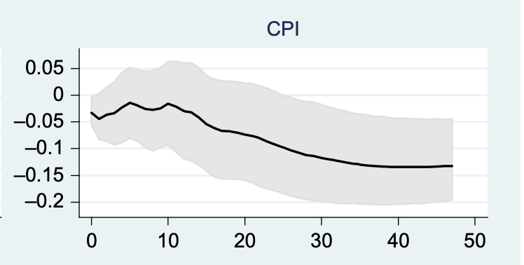
- Estimates disappear after 1982
Ramey’s first variation within the first plot is to make use of knowledge from 1983 to 2007. Her second variation is to additionally omit the financial variables. Christiano Eichenbaum and Evans had been nonetheless pondering when it comes to cash provide management, however our Fed doesn’t management cash provide.
The proof that larger rates of interest decrease inflation disappears after 1983, with or with out cash. This too is a standard discovering. It may be as a result of there merely are no financial coverage shocks. Nonetheless, we’re driving a automotive with a yellowed AAA street map dated 1982 on it.
Financial coverage shocks nonetheless appear to have an effect on output and employment, simply not inflation. That poses a deeper drawback. If there simply are no financial coverage shocks, we might simply get large customary errors on all the things. That solely inflation disappears factors to the vanishing Phillips curve, which would be the weak level within the principle to come back. It’s the Phillips curve by which decrease output and employment push down inflation. However with out the Phillips curve, the entire customary story for rates of interest to have an effect on inflation goes away.
- Computing long-run responses
The lengthy lags of the above plot are already fairly lengthy horizons, with fascinating economics nonetheless occurring at 48 months. As we get considering future neutrality, identification by way of future signal restrictions (financial coverage shouldn’t completely have an effect on output), and the impact of persistent rate of interest shocks, we’re considering even longer run responses. The “future dangers” literature in asset pricing is equally crucially considering future properties. Intuitively, we must always know this will probably be troublesome. There aren’t all that many nonoverlapping 4 yr durations after rate of interest shocks to measure results, not to mention 10 yr durations.
VARs estimate future responses with a parametric construction. Arrange the info (output, inflation, rate of interest, and so on) right into a vector (x_t = [y_t ; pi_t ; i_t ; …]’), then the VAR will be written (x_{t+1} = Ax_t + u_t). We begin from zero, transfer (x_1 = u_1) in an fascinating manner, after which the response operate simply simulates ahead, with (x_j = A^j x_1).
However right here an oft-forgotten lesson of Nineteen Eighties econometrics pops up: It’s harmful to estimate long-run dynamics by becoming a brief run mannequin after which discovering its long-run implications. Elevating matrices to the forty eighth energy (A^{48}) can do bizarre issues, the one hundred and twentieth energy (10 years) weirder issues. OLS and most probability prize one step forward (R^2), and can fortunately settle for small one step forward mis specs that add as much as large misspecification 10 years out. (I discovered this lesson within the “Random stroll in GNP.”)
Future implications are pushed by the utmost eigenvalue of the (A) transition matrix, and its related eigenvector. (A^j = Q Lambda^j Q^{-1}). This can be a profit and a hazard. Specify and estimate the dynamics of the mixture of variables with the most important eigenvector proper, and many particulars will be improper. However customary estimates aren’t making an attempt laborious to get these proper.
The “native projection” different immediately estimates future responses: Run regressions of inflation in 10 years on the shock immediately. You possibly can see the tradeoff: there aren’t many non-overlapping 10 yr intervals, so this will probably be imprecisely estimated. The VAR makes a powerful parametric assumption about long-run dynamics. When it is proper, you get higher estimates. When it is improper, you get misspecification.
My expertise working a number of VARs is that month-to-month VARs raised to giant powers usually give unreliable responses. Run no less than a one-year VAR earlier than you begin future responses. Cointegrating vectors are essentially the most dependable variables to incorporate. They’re sometimes the state variable that almost all reliably carries lengthy – run responses. However take note of getting them proper. Imposing integrating and cointegrating construction by simply items is a good suggestion.
The regression of long-run returns on dividend yields is an effective instance. The dividend yield is a cointegrating vector, and is the slow-moving state variable. A one interval VAR [left[ begin{array}{c} r_{t+1} dp_{t+1} end{array} right] = left[ begin{array}{cc} 0 & b_r 0 & rho end{array}right] left[ begin{array}{c} r_{t} dp_{t} end{array}right]+ varepsilon_{t+1}] implies a protracted horizon regression (r_{t+j} = b_r rho^j dp_{t} +) error. Direct regressions (“native projections”) (r_{t+j} = b_{r,j} dp_t + ) error give about the identical solutions, although the downward bias in (rho) estimates is a little bit of a difficulty, however with a lot bigger customary errors. The constraint (b_{r,j} = b_r rho^j) is not unhealthy. However it could actually simply go improper. If you happen to do not impose that dividends and value are cointegrated, or with vector apart from 1 -1, should you enable a small pattern to estimate (rho>1), should you do not put in dividend yields in any respect and simply lots of short-run forecasters, it could actually all go badly.
Forecasting bond returns was for me an excellent counterexample. A VAR forecasting one-year bond returns from immediately’s yields offers very completely different outcomes from taking a month-to-month VAR, even with a number of lags, and utilizing (A^{12}) to deduce the one-year return forecast. Small pricing errors or microstructure dominate the month-to-month knowledge, which produces junk when raised to the twelfth energy. (Local weather regressions are having enjoyable with the identical challenge. Small estimated results of temperature on progress, raised to the a hundredth energy, can produce properly calamitous outcomes. However use fundamental principle to consider items.)
Nakamura and Steinsson (appendix) present how delicate some customary estimates of impulse response capabilities are to those questions.
Weak proof
For the present coverage query, I hope you get a way of how weak the proof is for the “customary view” that larger rates of interest reliably decrease inflation, although with a protracted and variable lag, and the Fed has a great deal of management over inflation.
Sure, many estimates look the identical, however there’s a fairly robust prior getting in to that. Most individuals do not publish papers that do not conform to one thing like the usual view. Look how lengthy it took from Sims (1980) to Christiano Eichenbaum and Evans (1999) to provide a response operate that does conform to the usual view, what Friedman advised us to count on in (1968). That took lots of taking part in with completely different orthogonalization, variable inclusion, and different specification assumptions. This isn’t criticism: when you will have a powerful prior, it is smart to see if the info will be squeezed in to the prior. As soon as authors like Ramey and Nakamura and Steinsson began to look with a essential eye, it grew to become clearer simply how weak the proof is.
Normal errors are additionally broad, however the variability in outcomes as a consequence of adjustments in pattern and specification are a lot bigger than formal customary errors. That is why I do not stress that statistical side. You play with 100 fashions, strive one variable after one other to tamp down the value puzzle, after which compute customary errors as if the a hundredth mannequin had been written in stone. This submit is already too lengthy, however exhibiting how outcomes change with completely different specs would have been an excellent addition.
For instance, listed here are a number of extra Ramey plots of inflation responses, replicating numerous earlier estimates

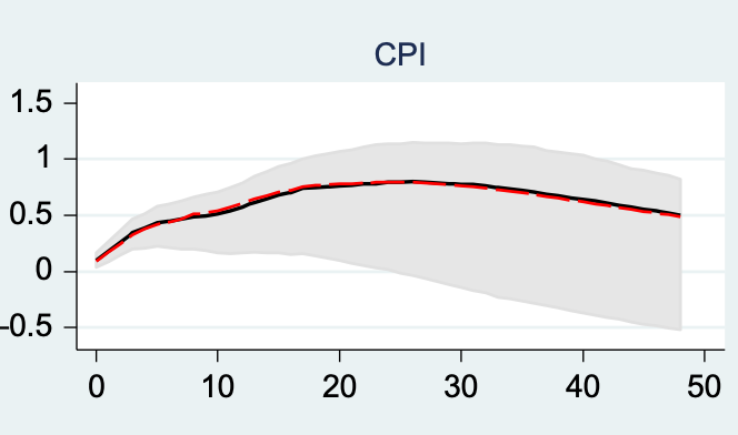

Take your choose.
What ought to we do as an alternative?
Properly, how else ought to we measure the results of financial coverage? One pure strategy turns to the evaluation of historic episodes and adjustments in regime, with particular fashions in thoughts.
Romer and Romer cross on ideas on this strategy:
…some macroeconomic habits could also be basically episodic in nature. Monetary crises, recessions, disinflations, are all occasions that appear to play out in an identifiable sample. There could also be lengthy durations the place issues are principally superb, which can be then interrupted by brief durations when they don’t seem to be. If that is true, one of the simplest ways to grasp them could also be to concentrate on episodes—not a cross-section proxy or a tiny sub-period. As well as, it’s worthwhile to know when the episodes had been and what occurred throughout them. And, the identification and understanding of episodes might require utilizing sources apart from typical knowledge.
Numerous my and others’ fiscal principle writing has taken an identical view. The lengthy quiet zero sure is a check of theories: old-Keynesian fashions predict a delation spiral, new-Keynesian fashions predicts sunspot volatility, fiscal principle is in step with steady quiet inflation. The emergence of inflation in 2021 and its easing regardless of rates of interest beneath inflation likewise validates fiscal vs. customary theories. The fiscal implications of abandoning the gold customary in 1933 plus Roosevelt’s “emergency” price range make sense of that episode. The brand new-Keynesian response parameter (phi_pi) in (i_t – phi_pi pi_t), which results in unstable dynamics for ](phi_pi>1) is just not recognized by time collection knowledge. So use “different sources,” like plain statements on the Fed web site about how they react to inflation. I already cited Clarida Galí and Gertler, for measuring the rule not the response to the shock, and explaining the implications of that rule for his or her mannequin.
Nakamura and Steinsson likewise summarize Mussa’s (1986) basic examine of what occurs when nations change from fastened to floating change charges:
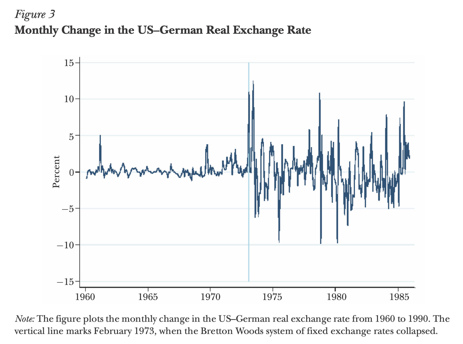
“The change from a hard and fast to a versatile change price is a purely financial motion. In a world the place financial coverage has no actual results, such a coverage change wouldn’t have an effect on actual variables like the actual change price. Determine 3 demonstrates dramatically that the world we dwell in is just not such a world.”
Additionally, evaluation of specific historic episodes is enlightening. However every episode has different issues occurring and so invitations different explanations. 90 years later, we’re nonetheless combating about what brought about the Nice Melancholy. 1980 is the poster baby for financial disinflation, but as Nakamura and Steinsson write,
Many economists discover the narrative account above and the accompanying proof about output to be compelling proof of enormous financial nonneutrality. Nonetheless, there are different potential explanations for these actions in output. There have been oil shocks each in September 1979 and in February 1981…. Credit score controls had been instituted between March and July of 1980. Anticipation results related to the phased-in tax cuts of the Reagan administration can also have performed a job within the 1981–1982 recession ….
Learning adjustments in regime, equivalent to fastened to floating or the zero sure period, assist considerably relative to learning a specific episode, in that they’ve a few of the averaging of different shocks.
However the attraction of VARs will stay. None of those produces what VARs appeared to provide, a theory-free qualitative estimate of the results of financial coverage. Many inform you that costs are sticky, however not how costs are sticky. Are they old-Keynesian backward wanting sticky or new-Keynesian rational expectations sticky? What’s the dynamic response of relative inflation to a change in a pegged change price? What’s the dynamic response of actual relative costs to productiveness shocks? Observations equivalent to Mussa’s graph can assist to calibrate fashions, however doesn’t reply these questions immediately. My observations concerning the zero sure or the current inflation equally appear (to me) decisive about one class of mannequin vs. one other, no less than topic to Occam’s razor about epicycles, however likewise don’t present a theory-free impulse response operate. Nakamura and Steinsson write at size about different approaches; model-based second matching and use of micro knowledge particularly. This submit is occurring too lengthy; learn their paper.
In fact, as now we have seen, VARs solely appear to supply a model-free quantitative measurement of “the results of financial coverage,” however it’s laborious to surrender on the looks of such a solution. VARs and impulse responses additionally stay very helpful methods of summarizing the correlations and cross correlations of information, even with out trigger and impact interpretation.
Ultimately, many concepts are profitable in economics after they inform researchers what to do, after they supply a comparatively clear recipe for writing papers. “Take a look at episodes and assume laborious is just not such recipe.” “Run a VAR is.” So, as you concentrate on how we are able to consider financial coverage, take into consideration a greater recipe in addition to an excellent reply.
(Keep tuned. This submit is prone to be up to date a number of instances!)
VAR technical appendix
Technically, working VARs may be very straightforward, no less than till you begin making an attempt to easy out responses with Bayesian and different strategies. Line up the info in a vector, i.e. (x_t = [i_t ; pi_t; y_t]’). Then run a regression of every variable on lags of the others, [x_t = Ax_{t-1} + u_t.] If you would like a couple of lag of the best hand variables, simply make a much bigger (x) vector, (x_t = [i_t; pi_t ; y_t ; i_{t-1}; pi_{t-1} ;y_{t-1}]’.)
The residuals of such regressions (u_t) will probably be correlated, so you must resolve whether or not, say, the correlation between rate of interest and inflation shocks means the Fed responds within the interval to inflation, or inflation responds inside the interval to rates of interest, or some mixture of the 2. That is the “identification” assumption challenge. You possibly can write it as a matrix (C) in order that (u_t = C varepsilon_t) and cov((varepsilon_t varepsilon_t’)=I) or you’ll be able to embody some contemporaneous values into the best hand sides.
Now, with (x_t = Ax_{t-1} + Cvarepsilon_t), you begin with (x_0=0), select one collection to shock, e.g. (varepsilon_{i,1}=1) leaving the others alone, and simply simulate ahead. The ensuing path of the opposite variables is the above plot, the “impulse response operate.” Alternatively you’ll be able to run a regression (x_t = sum_{j=0}^infty theta_j varepsilon_{t-j}) and the (theta_j) are (completely different, in pattern) estimates of the identical factor. That is “native projection”. Because the proper hand variables are all orthogonal, you’ll be able to run single or a number of regressions. (See right here for equations.) Both manner, you will have discovered the transferring common illustration, (x_t = theta(L)varepsilon_t), within the first case with (theta(L)=(I-AL)^{-1}C) within the second case immediately. Because the proper hand variables are all orthogonal, the variance of the collection is the sum of its loading on all the shocks, (cov(x_t) = sum_{j=0}^infty theta_j theta_j’). This “forecast error variance decomposition” is behind my assertion that small quantities of inflation variance are as a consequence of financial coverage shocks relatively than shocks to different variables, and largely inflation shocks.
Replace:
Luis Garicano has a terrific tweet thread explaining the concepts with a medical analogy.
* Some Papers: